
Application of automatic classifiers for condition monitoring of railway rolling stock
Aplicación de clasificadores automáticos a la monitorización de la condición de funcionamiento de material rodante ferroviario
E. Ruiz Torres 1, A. Bustos Caballero 2, H. Rubio Alonso 3, C. Castejón Sisamón 4.
Abstract
The evolution of technology towards the automation of industrial processes and the advances in interconnectivity have given way to what is known today as industry 4.0. These advances are of particular interest in the area of predictive maintenance of machines, where machine learning techniques have considerably improved condition diagnosis of machinery. This is of special importance in the railway industry, where maintenance constitutes an important part of its operating costs. This paper studies the application of machine learning techniques to vibration signals originating from a railway axle, tested on a railway test bench, through support vector machine algorithms for fault detection. A feature selection scheme composed of a series of sensitivity analyses is proposed in order to determine the best signal features for classification. The subsequent hyperparameter optimization proposed consists of a series of sensitivity analyses in order to determine the values of each parameter that result in a classifier with the most accuracy. Lastly, the effect of the location of the sensors in the axle from which the vibration signals are obtained is studied in order to determine their most apt configuration.
Keywords: Support vector machine, condition monitoring, vibrations, railway systems.
Resumen
La evolución tecnológica hacia la automatización de procesos industriales y los avances en la interconectividad han dado lugar a lo que conocemos como Industria 4.0. Un área particularmente beneficiada por estos avances tecnológicos es el mantenimiento predictivo de máquinas, donde la implementación de técnicas de aprendizaje automático ha mejorado considerablemente el diagnóstico de la condición de las mismas. Esto es especialmente sensible en el sector ferroviario, donde el mantenimiento constituye una parte importante de los costes de operación. En el presente trabajo se estudiará la aplicación de técnicas de aprendizaje automático a señales vibratorias procedentes de un eje ferroviario testeado en un banco de ensayos mediante algoritmos de máquinas de soporte vectorial para la detección de fallos. Con el propósito de obtener un clasificador preciso, se propone una selección de cualidades que consiste en una serie de análisis de sensibilidad con el propósito de determinar las mejores cualidades para la clasificación. La posterior optimización de hiperparámetros propuesta se constituye por una serie de análisis de sensibilidad, para determinar los valores de cada parámetro del clasificador que generan clasificadores con mayor precisión. Por último, se estudiará el efecto de la localización de los sensores de los que provienen las señales vibratorias para determinar su configuración más adecuada.
Palabras clave: Máquina de soporte vectorial, monitorización de la condición, vibraciones, sistemas ferroviarios.
Recibido/received: 01/06/2023 Aceptado/accepted: 10/10/2023
1 Dpto. de Ingeniería Mecánica. Universidad Carlos III de Madrid.
2 Dpto. de Mecánica. Universidad Nacional de Educación a Distancia.
3 Dpto. de Ingeniería Mecánica. Universidad Carlos III de Madrid.
4 Dpto. de Ingeniería Mecánica. Universidad Carlos III de Madrid.
Corresponding author: Enrique Ruiz Torres; e-mail: en*****@******3m.es
1. Introduction
The connectivity of today’s world penetrates all aspects of society where efficiency and the handling of data are of importance. This trend has manifested itself on an industrial level as the well-known industry 4.0, which is characterized by the automation of not only physical processes, but of intellectual processes as well, through the processing of large quantities of data (big data). Machine learning presents itself as a useful tool in the processing of this data. In line with this trend, predictive maintenance measures have been implemented through automatic classifiers capable of establishing condition monitoring systems of machinery in an efficient manner (Lee et al., 2014).
The railway sector stands out as an area of industry with potential to greatly benefit from these advances. Maintenance of railway infrastructure and rolling stock accounts for a significant part of its operating costs. Predictive maintenance using machine learning methods arises as a natural solution for the reduction of costs when the tendency of technological evolution of the sector and the recent advances in machine learning are considered (Bustos et al., 2021).
In consequence, the main objective of this work is the application of machine learning techniques for fault detection in railway rolling stock. In particular, Support Vector Machine (SVM) (Cortes & Vapnik, 1995) algorithms are used for the classification of vibration signals coming from a bogie test bench (Bustos et al., 2019) with defects of varying severity. These machine learning algorithms are based on the separation of observations in a space of high dimension using a hyperplane, with reasonable computational cost thanks to functions commonly referred to as kernels. SVMs are, fundamentally, binary classifiers, although multi-class classification can be achieved through codification techniques (Cristianini, 2000). SVMs have been shown to give good results in bearing fault detection through the classification of vibration signals (Rubio Alonso, s. f.; Sun & Liu, 2023).
In order to apply these techniques to vibration signals a previous signal feature selection must be performed in order to select the features that properly describe the condition of rolling stock. With this purpose in mind, a series of 21 signal features are proposed in time and frequency domain, and various classifiers are compared in order to determine the most apt features for classification. Then, the hyperparameters of the SVM are tuned in order to determine their values that are better suited for the classification of the selected features. A classification model and a set of signal features capable of fault detection in railway axles is meant to be obtained as a result of the previous procedures. Finally, the effect of the position of the sensors on the axle on classification is studied in order to determine its effect in the validity of the results.
2. Methodology
2.1. Experimental setup
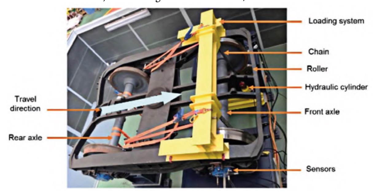
The vibration signals utilized come from a mechanical system which consists of a bogie test bench where a Y-21 Cse model bogie is mounted on two pairs of rollers. Hydraulic cylinders are used to activate the loading mechanism by means of a chain. The measurement system consists of three accelerometers mounted on each side of the axle box: One for the vertical direction, one for the axial direction and one for the direction of movement as can be seen in figure 1.
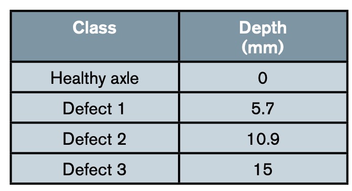
The axle defects are induced through radial machining at the centre of the axle. Four defect levels are defined ranging from no defect to a depth of 15 mm as can be seen in table 1.
The experimental tests consisted of rolling the front bogie wheels on the two rollers of the test bench, which dragged the wheels forward through friction (figure 1). The tests were carried out on the same bogie under similar operating conditions: at a speed of 50 km/h and an external load of 10 metric tons. The tests began with a healthy axle and the rest of the defect levels proposed in table 1 were progressively induced. The vibration signals were obtained sequentially during the course of each test.
2.2. Signal acquisition
The vibration signals used correspond to the acceleration signals obtained by the vertical accelerometers located on the axle boxes of the left and right-hand side of the front axle (fig. 1). Signals were recorded at a sampling rate of 12,800 Hz, up to a total of 16,384 samples (214), resulting in an acquisition time of 1.28 seconds. In this study, a total of 592 vibration records (9.7 million samples) were used, which include the four defect levels and the two sides of the axle:
•136 signals from the healthy axle (half on the right-hand side and the other half on the left-hand side).
•104 signals with defect 1 (half on the right-hand side and the other half on the left-hand side).
•144 signals with defect 2 (half on the right-hand side and the other half on the left-hand side).
•208 signals with defect 3 (half on the right-hand side and the other half on the left-hand side).
2.3. Classifier tests
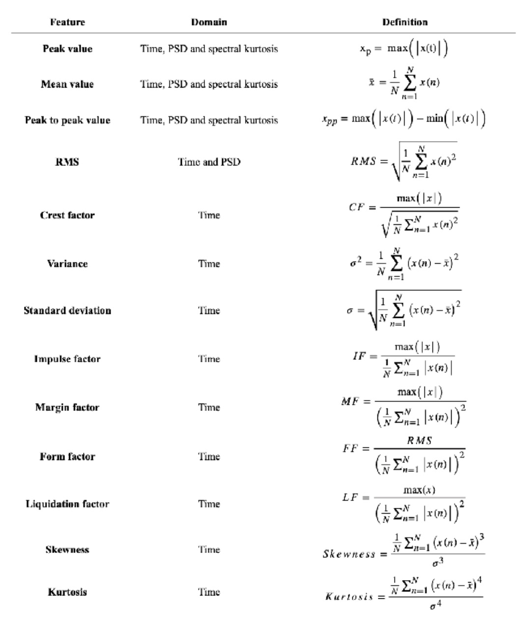
The accuracy of a classifier fundamentally depends on the ability of the input data to differentiate between the different classes. When considering fault detection through stationary vibration signals, statistical measures are commonly used as signal features, treating the signals as random variables (Randall, 2011). In this study, these measures are made up of a series of 13 statistical parameters, obtained from the vibration signals and the frequency spectrum, whose detailed descriptions are laid out in table 2.
For the frequency domain features, the power spectral density (PSD) spectrum is used. In addition, features of the spectral kurtosis spectrum are evaluated; a tool that allows for the filtering of regions with Gaussian noise, facilitating the detection of parts of the signal with relevant information (Antoni, 2006). The spectral kurtosis spectrum has been shown to give good results in fault detection using vibration signals due to its ability to separate noise from characteristic impulses of faults in rotary machines (Antoni & Randall, 2006). In total, 21 features are considered (12 in time domain, 5 from the PSD spectrum and 3 from the spectral kurtosis spectrum).
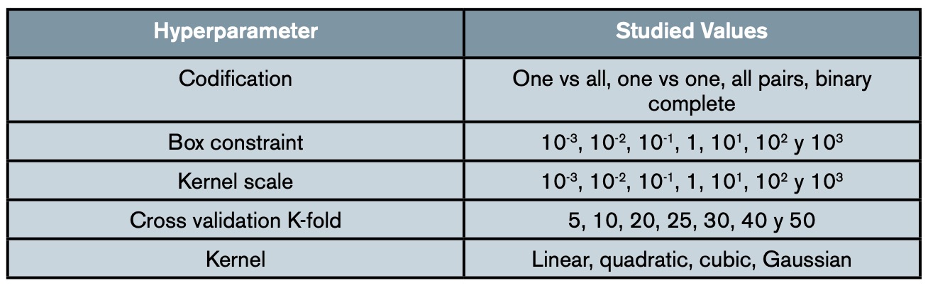
Once the features are defined, a sensitivity analysis is carried out to evaluate their aptitude in classification. This analysis consists of training several classifiers with each feature individually and varying their hyperparameters to take their effect into account. The purpose is to obtain a measure of the aptitude of each individual feature independent of the parameters of the final classifier. The sensitivity analyses are carried out with four hyperparameters and four kernels, whose range of values studied can be seen in table 3.
In order to identify the hyperparameters that generate classifiers with high accuracy, a subsequent hyperparameter study is carried out. This study consists of a series of sensitivity analyses, similar to those carried out for the feature selection, according to table 3, with the distinction of using a classifier trained with all the previously selected features.
2.4. Study of sensor position
The location of the measurement sensor on the axle affects the vibration signals obtained and, therefore, it also affects the values of its features. In order to identify the significance of this effect, a study of sensor location is carried out. To perform this study, the analyses described in the previous section are carried out concurrently both for signals taken from the left side of the axis (LHS signal set) and from the right side (RHS signal set). In addition, the possibility of combining the signals in two different configurations is considered:
1. Mixed sides (MS signal set): a combination of signals from the left and right-hand side of the axle is used, without any feature that directly identifies them as such. 2.Identified mixed sides (IMS signal set): a combination of signals from the left and right-hand side of the axle is used, incorporating the sensor from which each signal comes from (LHS or RHS) as an additional feature.
This last study is carried out during the tuning of hyperparameters, meaning that the classifiers trained on these last two signal sets use the same features for classification as the classifiers trained with the signals from the LHS and RHS signal sets.
3. Results
Once the vibration signals have been obtained and after the necessary feature extraction has been performed, the classifier tests are carried out. The feature extraction and the implementation of the SVM algorithm are implemented in the commercial program Matlab, using its Classification Learner application from the Statistics and Machine Learning Toolbox.
3.1. Feature selection
The sensitivity analysis for the feature selection is repeated for four hyperparameters and four kernels, resulting in 16 accuracy values for each feature studied. Although absolute variation in accuracy is observed among different tests, no significant variation is seen for the relative values between features with equal hyperparameters. That is, the different analyses gave rise to the same set of selected features.
For simplicity, and due to the similarity of results, the analysis with varying box constraint is discussed as it is the most representative case. The conclusions obtained can, however, be extrapolated to the rest of the analyses. This test was carried out with a kernel scale value of 1, one vs. one codification and cross validation with a k-fold value of 5. The results presented in tables 4 and 5 correspond to the average accuracy of the four kernels studied for the LHS and RHS sets respectively.
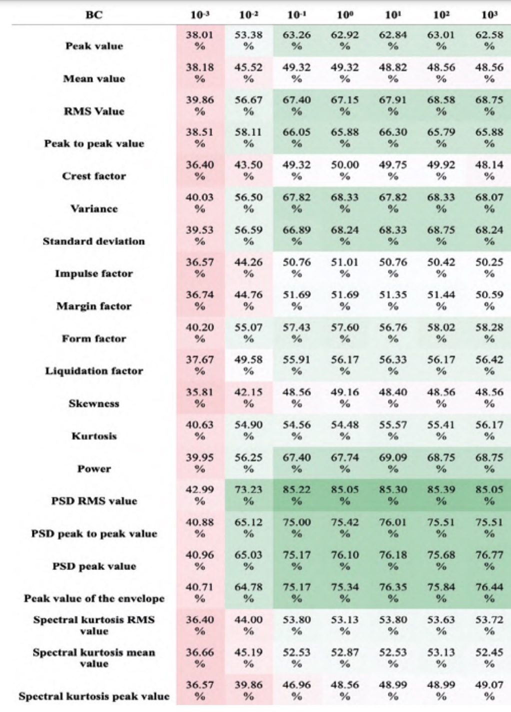
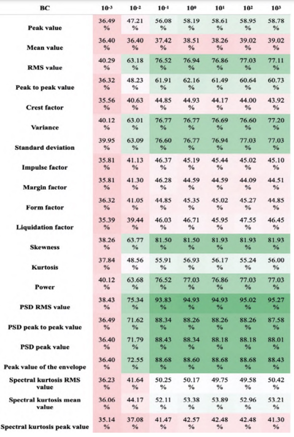
In tables 4 and 5 it can be seen that the features associated with the PSD are considerably better performant for classification than the rest of the features, corroborating the results obtained in previous studies (Bustos et al., 2019). Among the features of the PSD, the RMS value stands out, which achieves maximum accuracy in all cases. Taking the high range of hyperparameters studied into account, it is considered appropriate to conclude that the RMS value of the PSD will be highly significant, regardless of the hyperparameters of the final classifier.
Among the time domain features, the following stand out: the RMS value, the variance and standard deviation, and the skewness. It is possible that the high performance of the RMS value is associated with the information it provides about the signal power, as it can be seen in tables 4 and 5 by the correlation between the accuracies of the power and the RMS value. The variance and standard deviation also stand out, possibly due to the information they provide about the variability of the signal and, therefore, the interference of the vibrations generated by the fault. The correlation between their values is evident since one is mathematically defined as the square root of the other (table 2). Finally, the skewness value is particularly effective for classifying signals from the RHS set, although it is not significant in the LHS set.
In light of the results analysed above, six features were selected for classification with high accuracy and without correlation between each other:
•Peak value of the time signal.
•RMS value of the time signal.
•Variance of the time signal.
•Skewness of the time signal.
•RMS of the power spectrum.
•Peak value of the power spectrum
3.2. Tuning of Hyperparameters
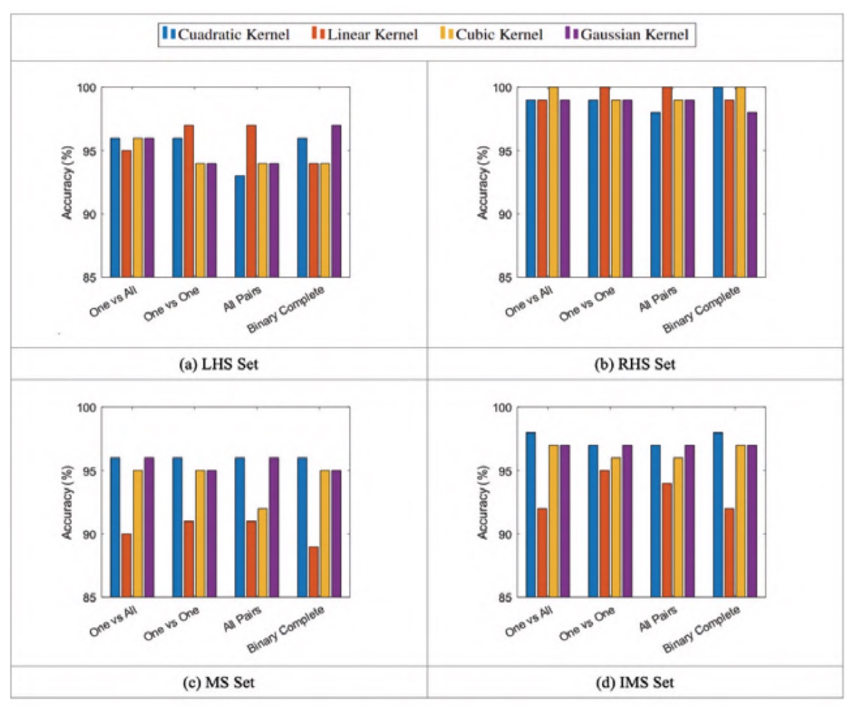
Similar to the studies carried out for the feature selection, sensitivity analyses are performed for four hyperparameters and four kernels. In this case the classifiers are trained with the set of features previously selected. Additionally, the hyperparameters for the MS and IMS sets are also tuned.
Little variation in accuracy can be seen for different codifications, as can be seen in figure 2. The maximum accuracy is obtained with different kernels, depending on the training set (LHS, RHS, LM or LMI). Their distribution relative to different kernels, however, remains relatively constant between signal sets except in the case of the LHS set, in which an increase in the variability of the quadratic and Gaussian kernels is observed.
Figure 3 shows how the signal accuracies of the LHS and RHS sets vary almost identically with the box constraint, reaching higher maximum accuracies in the RHS set. The accuracy of the MS and IMS sets behave similarly, with the IMS set showing marginally higher accuracies.
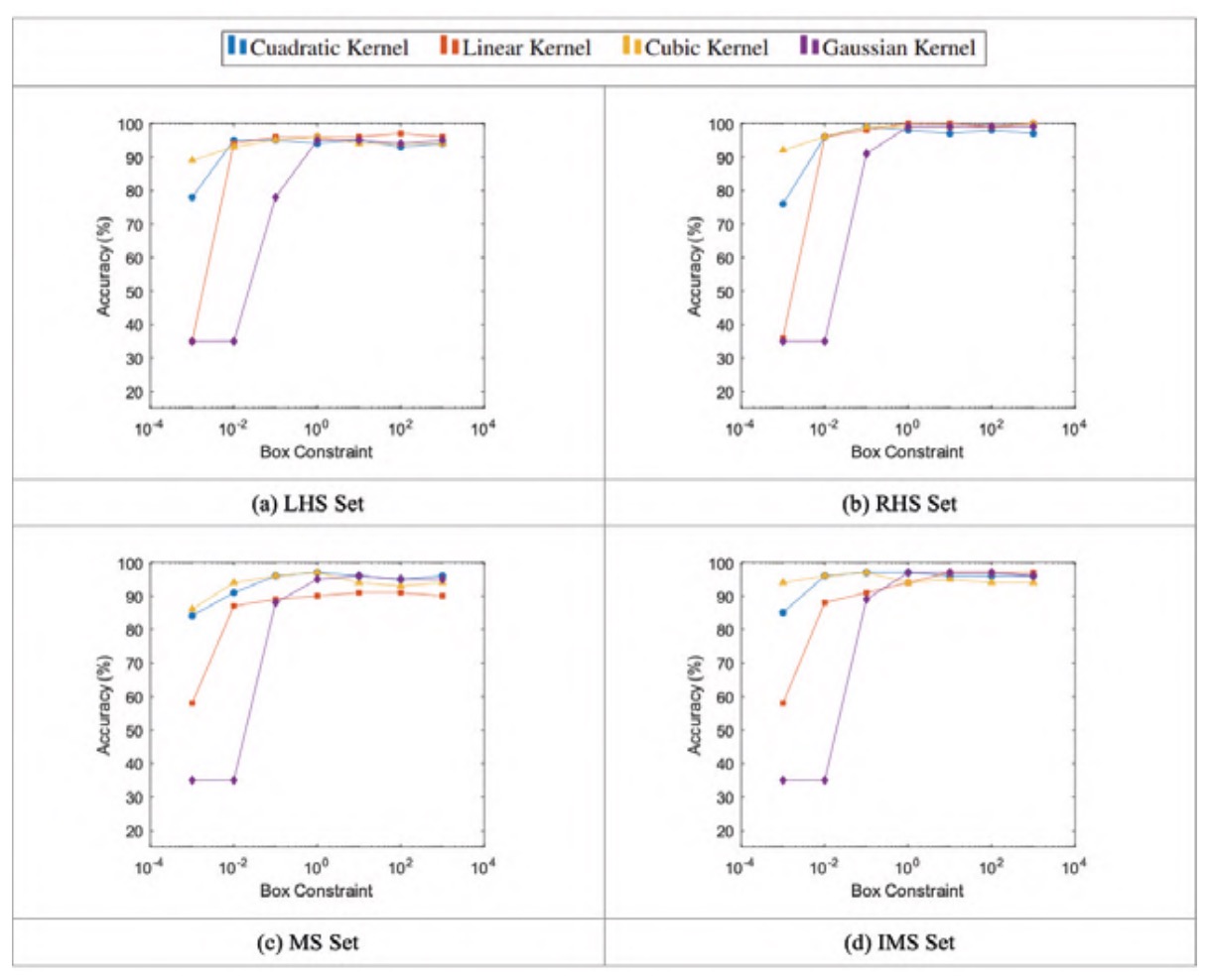
Figure 3 also shows that small values of the box constraint give comparatively low accuracy values, with the linear and Gaussian kernels being particularly susceptible to this effect. As the box constraint increases, all kernels converge to a similar accuracy value, beginning to converge at a box constraint value of approximately 10-2 for the quadratic, linear and cubic kernels and a box constraint value of approximately 1 for the Gaussian kernel.
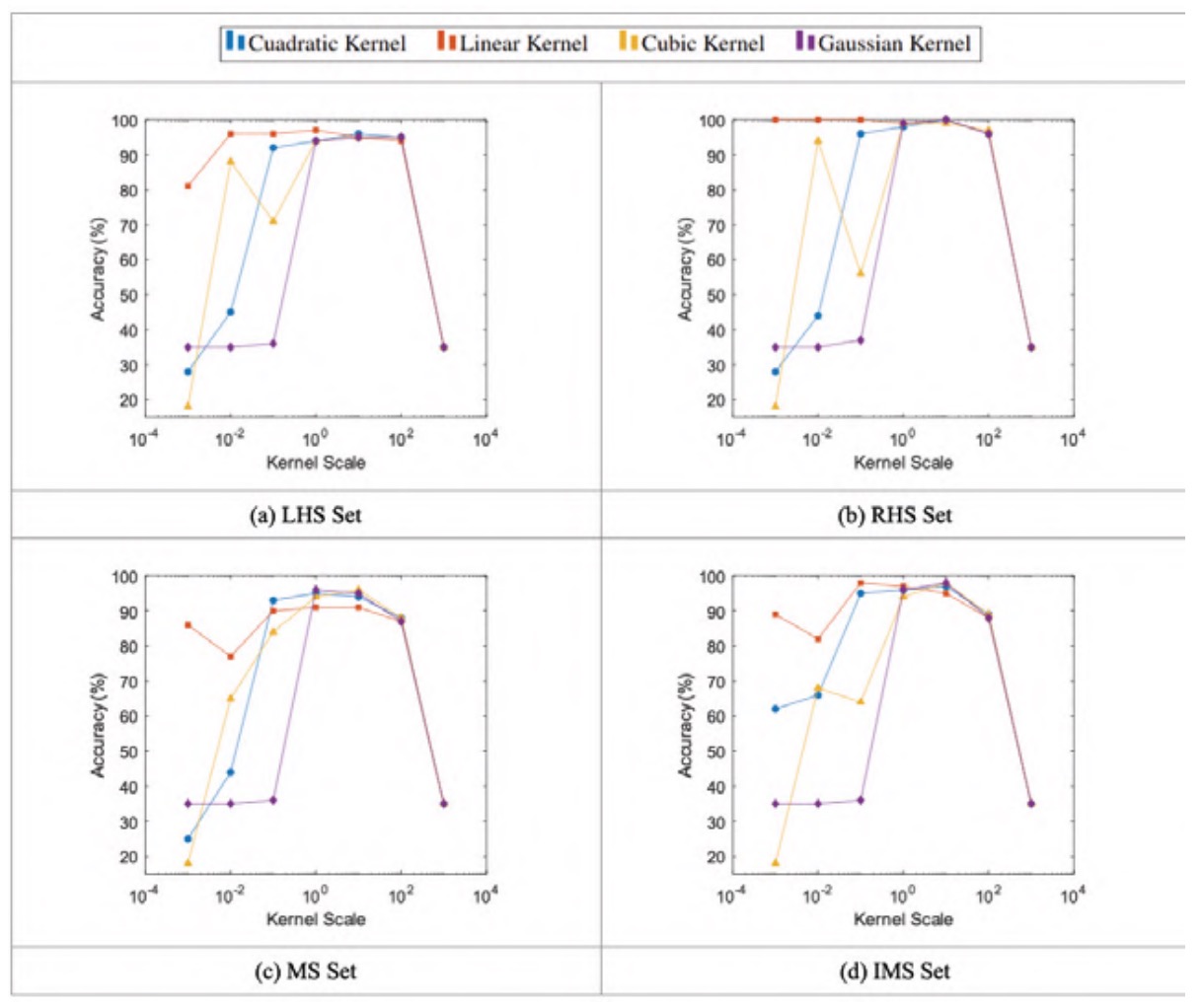
In similarity to the case of the box constraint, figure 4 shows how small values of the kernel scale result in low accuracy values. This behaviour holds for all kernels, except for the linear kernel, which maintains comparatively high accuracy values. It can be seen that the accuracies do not converge, but rather reach a maximum with kernel scale values between 1 and 10.
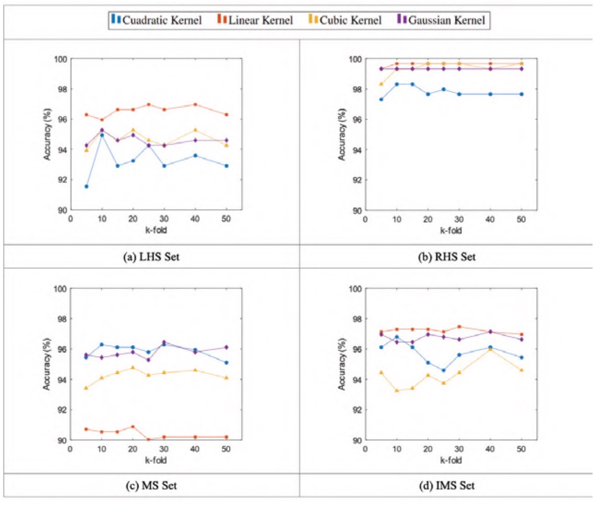
Figure 5 shows how, as with the codification case, there appears to be no significant variation in accuracy values between high and low values of the k-fold. On the other hand, the accuracy remains relatively constant, oscillating around an average value. The quadratic kernel has greater variability, while the Gaussian kernel is the most constant.
The linear kernel stands out for its high accuracy relative to other kernels in most cases, with the exception of the MS set, in which the lowest accuracies are obtained. The cubic kernel obtains comparatively high accuracy values for the LHS and RHS signal sets, although low accuracy values are obtained for the MS and IMS signal sets. The quadratic kernel behaves in the opposite way, obtaining low accuracy values for the LHS and RHS signal sets and high accuracy values for the MS and IMS signal sets. The Gaussian kernel, on the other hand, does not vary significantly relative to other kernels. This difference in behaviour between signal sets seems to indicate that the appropriate kernel and hyperparameter values depend on the set of signals used for training, as was the case with the feature selection.
3.3. Study of sensor position
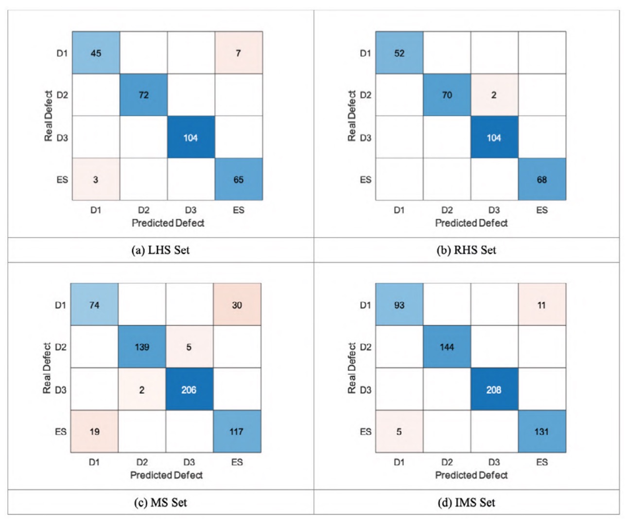
In figure 6, as an illustrative example, confusion matrices for the classifiers corresponding to each sensor configuration are presented and discussed for the case of one vs one coding, box constraint of 100, kernel scale of 1, cross validation with k-fold value of 5 and linear kernel.
Figure 6 shows how the main loss of accuracy for the classifier with the LHS set can be interpreted as the confusion between the healthy axle (ES) and defect 1 (D1) classes. In the case of the RHS set, the loss of accuracy is due to the confusion between defect 2 (D2) and defect 3 (D3). The increase in accuracy could possibly be explained by the high classification ability of the skewness of the time signal for the RHS signal set, as discussed in the feature selection section. The two matrices are mainly diagonal, although the RHS set classifier achieves the highest accuracy. It can be deduced, therefore, that the behaviour of the signals during classification depends on the location of the sensor.
The classifier for the MS signal set has the lowest performance of the four cases. Figure 6 shows how, in addition to the confusion between the healthy axle and defect 1, there is some confusion between defect 2 and defect 3. A possible explanation for the decrease in accuracy is that the combination of the LHS and RHS sets gives rise to a set of signals without a clear distinction between classes, possibly due to the differences between the separation of classes of the LHS and RHS sets previously discussed.
Lastly, figure 6 shows how the IMS signal set classifier behaves almost identically to the LHS signal set classifier. Again, the main cause of the loss of accuracy is due to the confusion between the healthy axle and defect 1. This seems to indicate that the identification of the signals is effective in eliminating the effect that generates the loss of accuracy in the case of the MS signal set. 4.
Conclusions
The main objective of this work was the application of machine learning techniques, through the use of support vector machine algorithms, for the classification of vibration signals for the fault detection in railway rolling stock. For this purpose, several vibration signals were recorded, coming from a bogie test bench where tests were carried out with healthy axles and with different levels of defects. Once the signals were recorded, a series of sensitivity analyses were carried out to select features and hyperparameters capable of classifying the signals effectively. In light of the results obtained, it can be concluded that the methodology followed is capable of generating high-accuracy classifiers: in some classifiers, accuracies of 100% have been achieved.
With regards to the feature selection, it is concluded that the best features for classification are those associated with the spectral power density spectrum. It is also concluded that the set of features to be selected is independent of the hyperparameters of the final classifier. However, they do depend on the set of signals used in training, as has been seen with the difference in accuracy provided by the signal skewness between the sets on the left and right-hand side of the axle.
In relation to the tuning of hyperparameters, it is concluded that there is a strong relationship between the appropriate hyperparameters and the kernel used. Some variation is also observed for different sets of signals: the accuracies of classifiers seem to be independent of the values of both the codification and the k-fold of the cross-validation, with the kernel and signal set used in training being the dominant factors in these cases. It can also be concluded that both very low values of the box constraint and very low or high values of the kernel scale result in classifiers with low accuracy in general. After analysis, it is deduced that an appropriate value for these parameters ranges between 10-1 and 102 .
With regards to the analysis of the sensor location, it is concluded that the location of the sensors plays an important role in fault detection through vibration signals since it has an important impact on the feature selection, hyperparameter tuning and classification. It is also noted that mixing signals originating from different sensors without discriminating between signal sets results in a less accurate classifier overall, although this effect can be somewhat mitigated by incorporating an additional feature that identifies which sensor each signal originates from.
5. Acknowledgements
This publication is part of Project I+D+I MC 4.0, financed by AEI/10.13039/501100011033 though subprojects PID2020-116984RB-C21 and PID2020-116984RB-C22.
References
Antoni, J. (2006). The spectral kurtosis: A useful tool for characterising nonstationary signals. Mechanical Systems and Signal Processing, 20(2), 282-307.
Antoni, J., & Randall, R. B. (2006). The spectral kurtosis: Application to the vibratory surveillance and diagnostics of rotating machines. Mechanical Systems and Signal Processing, 20(2), 308-331.
Bustos, A., Rubio, H., Meneses, J., Castejon, C., & Garcia-Prada, J. C. (2019). Crack detection in freight railway axles using Power Spectral Density and Empirical Mode Decomposition Techniques. Advances in Mechanism and Machine Science, 73, 3691-3701.
Bustos, A., Rubio, H., Soriano-Heras, E., & Castejon, C. (2021). Methodology for the integration of a high-speed train in Maintenance 4.0. Journal of Computational Design and Engineering, 8(6), 1605-1621.
Cortes, C., & Vapnik, V. (1995). Supportvector networks. Machine Learning, 20(3), 273-297.
Cristianini, N. (2000). An introduction to support vector machines: And other Kernel-based learning methods. Cambridge University Press.
Junquera, E., Rubio, H., Bustos, A. & Soriano, E. Aplicación de Técnicas de Aprendizaje Automático a la Diagnosis de Sistemas Mecánicos [Conference paper presentation]. XV Congreso Iberoamericano de Ingeniería Mecánica, Madrid. (2022, november 22-24).
Lee, J., Wu, F., Zhao, W., Ghaffari, M., Liao, L., & Siegel, D. (2014). Prognostics and health management design for rotary machinery systems—Reviews, methodology and applications. Mechanical Systems and Signal Processing, 42(1-2), 314-334.
Randall, R. B. (2011). Vibration-based condition monitoring: Industrial, aerospace, and automotive applications. Wiley.
Sun, B., & Liu, X. (2023). Significance Support Vector Machine for HighSpeed Train Bearing Fault Diagnosis. IEEE Sensors Journal, 23(5), 4638- 4646.